[an error occurred while processing this directive] [an error occurred while processing this directive]

Solution of the Black Scholes Equation

Key Concepts

1. The Black-Scholes equation for the value of a European call option on a security can be solved by judicious changes of variables that reduce the equation to the heat equation, for which we can write down the solution.
2. An example of how to choose and execute changes of variables to solve a partial differential equation.

Vocabulary

1. A differential equation with auxiliary initial conditions and boundary conditions, that is an initial value problem, is said to be well-posed if the solution exists, is unique, and small changes in the equation parameters, the initial conditions or the boundary conditions produce only small changes in the solutions.

Mathematical Ideas

Analytic Solution of the Black-Scholes Equation

This discussion is drawn from Section 4.2, pages 59-63; Section 4.3, pages 66-69; Section 5.3, pages 75-76; and Section 5.4, pages 77 - 81 of The Mathematics of Financial Derivatives: A Student Introduction by P. Wilmott, S. Howison, J. Dewynne, Cambridge University Press, Cambridge, 1995. Some ideas are also taken from Chapter 11 of Stochastic Calculus and Financial Applications by J. Michael Steele, Springer, New York, 2001.

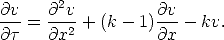
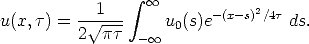
We have to start somewhere, and to avoid the problem of deriving everything back to calculus, we will assert that the initial value problem for the heat equation on the infinite interval is well-posed, that is, the solution to the partial differential equation

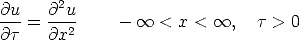
with

where the initial condition and the solution satisfy the following technical requirements:

1. u₀(x) has no more than a finite number of discontinuities of the jump kind,
2. lim _|x|u₀(x)e^-ax2 = 0 for any a > 0,
3. lim _|x|u(x,)e^-ax2 = 0 for any a > 0

exists for all time, is unique, and most importantly, can be represented as

Remark: This solution can derived in several different ways, I think the easiest way is to use Fourier transforms. The derivation of this solution representation is standard in any course or book on partial differential equations.

Remark: Mathematically, the conditions above are unnecessarily restrictive, and can be considerably weakened, however, they will be more than sufficient for all practical situations we encounter in mathematical finance.

Remark: The use of for the time variable (instead of the more natural t) is to avoid a conflict of notation in the several changes of variables we will soon have to make.

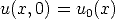
The Black-Scholes terminal value problem for the value V (S,t) of a European call option on a security with price S at time t is

with V (0,t) = 0, V (S,t) ~ S as S and

Note that this looks a little like the heat equation on the infinite interval in that it has a first derivative of the unknown with respect to time and the second derivative of the unknown with respect to the other (space) variable, but notice:

1. Each time the unknown is differentiated with respect to S, it also multiplied by the independent variable S, so the equation is not a constant coefficient equation.
2. There is a first derivative of V with respect to S in the equation.
3. There is a zero-th order term V in the equation.
4. The sign on the second derivative is the opposite of the heat equation form, so the equation is of backward parabolic form.
5. The data of the problem is given at the final time T instead of the initial time 0, consistent with the backward parabolic form of the equation.
6. There is a boundary condition V (0,t) = 0 specifying the value of the solution at one sensible boundary of the problem. The boundary is sensible since security values must only be zero or positive. This boundary condition says that any time the security value is 0, then the call value (with strike price K) is also worth 0.
7. There is another boundary condition V (S,t) ~ S, as S , but although this is financially sensible, (it says that for very large security prices, the call value with strike price K is approximately S) it is more in the nature of a technical condition, and we will ignore it without consequence.

We will eliminate each and every one of these objections with a suitable change of variables. The plan is to change variables to reduce the Black-Scholes terminal value problem to the heat equation, and then to use the known solution of the heat equation to represent the solution, and change variables back. This is a standard technique of solution in partial differential equations, and none of the transformations we are making are strange, unmotivated, or unknown.

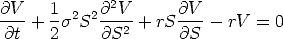
First we will take t = T - and S = Ke^x, and we will set

Remember, is the volatility, r is the interest rate on a risk-free bond, and K is the strike price. In the changes of variables above, the choice for t reverses the sense of time, changing the problem from backward parabolic to forward parabolic. The choice for S is a well-known transformation based on experience with the Euler equidimensional equation in differential equations. In addition, the variables have been carefully scaled so as to make the transformed equation expressed in dimensionless quantities. All of these techniques are standard and are covered in most courses and books on partial differential equations and applied mathematics.

Some extremely wise advice adapted from page 186 of Stochastic Calculus and Financial Applications by J. Michael Steele. Springer, New York, 2001 is appropriate here.

Following our advice, we first have to write

and

so

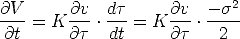
and

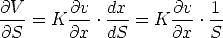
and

and the terminal condition

but V (S,T) = Kv(x, 0) so v(x, 0) = max(e^x - 1, 0).

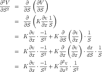
Now substitute all of the derivatives into the Black-Scholes equation to obtain:

Now the simplification begins:

1. Factor the common factor K and cancel.
2. Transpose the -derivative to the other side, and divide through by ²/2
3. Rename the remaining constant r/(²/2) as k. k measures the ratio between the risk-free interest rate and the volatility.
4. Cancel the S² terms in the second derivative.
5. Cancel the S terms in the first derivative.
6. Gather up like order terms.

What remains is the rescaled, constant coefficient equation:

We have made considerable progress, because

1. Now there is only one dimensionless parameter k measuring the risk-free interest rate as a multiple of the volatility and another (more or less hidden) rescaled time to expiry (1/2)²T , not the original 4 dimensioned quantities, namely K, T, ² and r.
2. The equation is defined on the interval - < x < , since this x-interval defines 0 < S < through the change of variables S = Ke^x.
3. The equation is now constant coefficient. In principle, we could solve the equation directly now,

Instead, we will change the dependent variable scale yet again, by

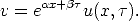
where and are yet to be determined. Now using the product rule:

and

and

Put these into our constant coefficient partial differential equation, cancel the common factor of e^x+ throughout and obtain:

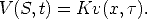
Now gather like terms:

Then choose = -(k - 1)/2 so that the u_x coefficient is 0, and then choose = ² + (k - 1) - k = -(k + 1)²/4 so the u coefficient is likewise 0. With this choice, the equation is reduced to

We also need to transform the initial condition too. This would be

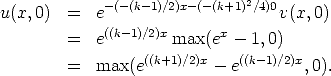
For future reference, we notice that this function is strictly positive when the argument x is strictly positive, that is u₀(x) > 0 when x > 0, otherwise, u₀(x) = 0 for x < 0.

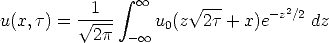
Now we are in the final stage, since we are ready to apply the solution representation formula:

However, first we want to make a change of variable in the integration, by taking z = (s - x)/, (and thereby dz = (-1/) dx) so that the integration becomes:

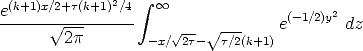
We may as well only integrate over the domain where u₀ > 0, that is for z > -x/. On that domain, u₀ = e^{((k+1)/2)(x+z)} - e^{((k-1)/2)(x+z)} so we are down to:

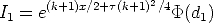
Call the two integrals I₁ and I₂ respectively.

We will evaluate I₁ ( the one with the k + 1 term) first. This is easy, just completing the square in the exponent yields a standard, tabulated integral. The exponent is

Therefore

Now, change variables again on the integral, choosing y = z -(k + 1) so dy = dz, and all we need to change are the limits of integration:

The integral can be represented in terms of the cumulative distribution function of a normal random variable, typically denoted . That is,

so

where d₁ = x/ + (k + 1) (note the use of the symmetry of the integral!) The calculation of I₂ is identical, except that (k + 1) is replaced by (k - 1) throughout.

That, is the solution of the heat equation is

where d₁ = x/ + (k + 1) and d₂ = x/ + (k - 1).

Now, we must systematically unwind each of the changes of variables, from u, first v(x,) = e^{(-1/2)(k-1)x-(1/4)(k+1)2}u(x,). (Notice how many of the exponentials neatly combine and cancel!) Then put x = log(S/K), = (1/2)²(T - t) and V (S,t) = Kv(x,).

The final solution is the Black-Scholes formula for the value of a European call option at time T with strike price K, if the current time is t and the underlying security price is S, the risk-free interest rate is r and the volatility is :

Note, usually one doesn’t see the solution as this full closed form solution. Instead, most versions of the solution write intermediate steps in small pieces, and then present the solution as an algorithm putting the pieces together to obtain the final answer.

Graphical Solution of the Black-Scholes Equation

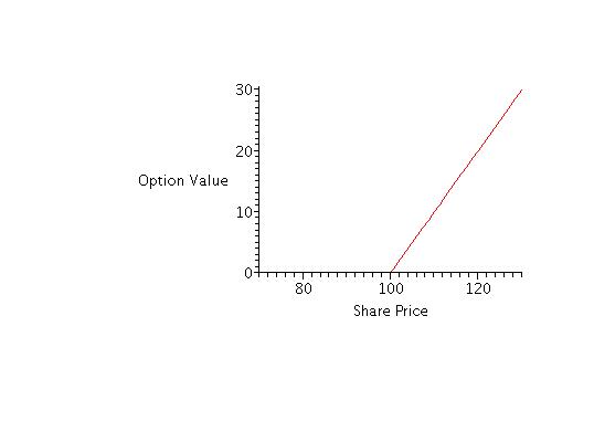
Consider for purposes of graphical illustration the value of a call option with strike price K = 100. The risk-free interest rate per year, continuously compounded is 12%, so r = 0.12, the time to expiration is T = 1 measured in years, and the standard deviation per year on the return of the stock, or the volatility is . The value of the call option at maturity plotted over a range of stock prices 70 < S < 130 surrounding the strike price is illustrated below:

Now, we use the Black-Scholes formula above to compute the value of the option prior to expiration. With the same parameters as above the value of the call option is plotted over a range of stock prices 70 < S < 130 at time remaining to expiration t = 1 (red), t = 0.8, (orange), t = 0.6 (yellow), t = 0.4 (green), t = 0.2 (blue) and at expiration t = 0 (black).

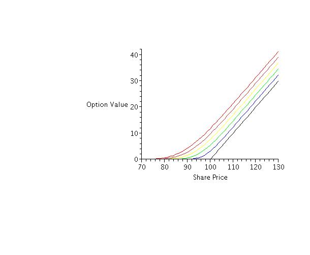
Notice a couple of trends in the value from this graph:

1. As the stock price increases, for a fixed time the option value increases,
2. As the time to expiration decreases, for a fixed stock value price the value of the option decreases to the value at expiration.

We can also plot the solution of the Black-Scholes equation as a function of security price and the time to expiration as value surface:

Problems to Work for Understanding

1. Explicitly evaluate the integral I₂ in terms of the c.d.f. and other elementary functions as was done for the integral I₁.

   Solution

2. What is the price of a European call option on a non-dividend-paying stock when the stock price is $52, the strike price is $50, the risk-free interest rate is 12% per annum (compounded continuously), the volatility is 30% per annum, and the time to maturity is 3 months?

   Solution

3. What is the price of a European call option on a non-dividend paying stock when the stock price is $30, the exercise price is $29, the risk-free interest rate is 5%, the volatility is 25% per annum, and the time to maturity is 4 months?

   Solution

4. Show that the Black-Scholes formula for the price of a call option tends to max(S - K, 0) as t T.

   Solution

Reading Suggestion:

1. Section 4.2, pages 59-63; Section 4.3, pages 66-69; Section 5.3, pages 75-76; and Section 5.4, pages 77 - 81 of The Mathematics of Financial Derivatives: A Student Introduction by P. Wilmott, S. Howison, J. Dewynne, Cambridge University Press, Cambridge, 1995.
2. Chapter 11 of Stochastic Calculus and Financial Applications by J. Michael Steele. Springer, New York, 2001.

Outside Readings and Links:

1. Cornell University , Department of Computer Science, Prof. T. Coleman Rhodes and Prof. R. Jarrow, Numerical Solution of Black-Scholes Equation, Submitted by Chun Fan, Nov. 12, 2002.
2. Monash University , Department of Mathematical Science, Eric. W. Chu Applied mathematicians transform the Black-Scholes Equation into a simpler forward form and solve it.It gives some examples and maple commands, Submitted by Chun Fan, Nov. 12, 2002.
3. ¡/a¿ An applet for calculating the option value based on Black-Scholes model. Also contains tips on options, business news and literature on options. Submitted by Yogesh Makkar, November 19, 2003.
4. ExcelEverywhere, a commercial application for spreadsheets on the Web A sample spreadsheet based calculator for calculating the option values, based on Black-Scholes model. Submitted by Yogesh Makkar, November 19,2003

[an error occurred while processing this directive] [an error occurred while processing this directive]

Last modified: [an error occurred while processing this directive]