[an error occurred while processing this directive] [an error occurred while processing this directive]

Question of the Day

Key Concepts

1. The probability of an event A conditional on another event B is generally different from the probability of B conditional on A. However, there is a definite relationship between the two, and Bayes’ theorem is the statement of that relationship. (Statement adapted from Wikipedia.)

Vocabulary

1. The law of total probability
2. Bayes Theorem says

Mathematical Ideas

Bayes’ theorem is named after the Reverend Thomas Bayes (1702-1761), who studied how to compute a distribution for the parameter of a binomial distribution (to use modern terminology). His friend, Richard Price, edited and presented the work in 1763, after Bayes’ death, as An Essay towards solving a Problem in the Doctrine of Chances. Pierre-Simon Laplace replicated and extended these results in an essay of 1774, apparently unaware of Bayes’ work.

This section is adapted from: Bayes theorem, in the Wikipedia.

Bayes Theorem

Bayes Theorem allows us to calculate the probability of an event when the universe can be partitioned into two or more disjoint parts.

Some times this statement is known as the law of total probability. The law of total probability says that the probability of an event E is a weighted average of the conditional probability of E given that even t A_i has occurred over all the total possibilities of A_i.

This formula can be helpful if it is difficult to calculate directly, but it can be computed with additional information about .

If 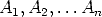form a partition of the sample space and E is an event of the sample space then Bayes Theorem says

Reversing Conditional Probabilities with Bayes Theorem

This section is adapted from: The Heart of Mathematics, 1st Edition, by E. B. Burger and Michael Starbird, Key Curriculum Press, 2000, page 614, problems II. 6,

An eyewitness observes a hit-and-run taxi-cab accident in a city in which 95% of the cabs are green and 5% are blue. The witness is 80% sure the cab was blue. Given all this information, how likely is it that the cab actually was blue?

Answer: One way to answer this question is imagine a universe of 1000 randomly staged accidents observed by this hypothetical observer. In 950 of these accidents, the taxi-cab would be green, and in 50 of these accidents the taxicab would be blue. By the observer being 80% sure, let us interpret that as 80% of the time the observer observes and recalls the cab color correctly and in 20% cases the observer recalls incorrectly the cab color. Among the 50 accidents with a blue cab, the observer would recall 40 of them correctly, and 10 of them incorrectly as being a green cab. Furthermore, the observer would recall 760 of them correctly as occurring with a green cab, and 190 of those accidents as occurring with a blue cab! Hence, if the observer insists that the accident occurred with a blue, then it did occur with a blue cab in 40/(40 + 190) = 0.173 or about 17% of the time. Adding an only somewhat reliable eyewitness adds only slightly to our belief about the color of the cab!

This problem is an application of Bayes’ formula for inverting conditional probabilities: Let B be the even that a Blue cab staged the hit and run accident. Let EB be the probability that the Eyewitness reported a Blue cab. Then the complementary event is EG, the Eyewitness reports a Green taxicab, so that the entire universe of event is contained in . Then we know that Pr[EB|B] = 0.8 and Pr[EG|G] = 0.8, because the eyewitness is 80% accurate. Hence Pr[EB|G] = 0.2, again because the eyewitness is 80% reliable.

This is the same arithmetic as the previous example with 1000 cases.

Here is a tree diagram of the same calculations:

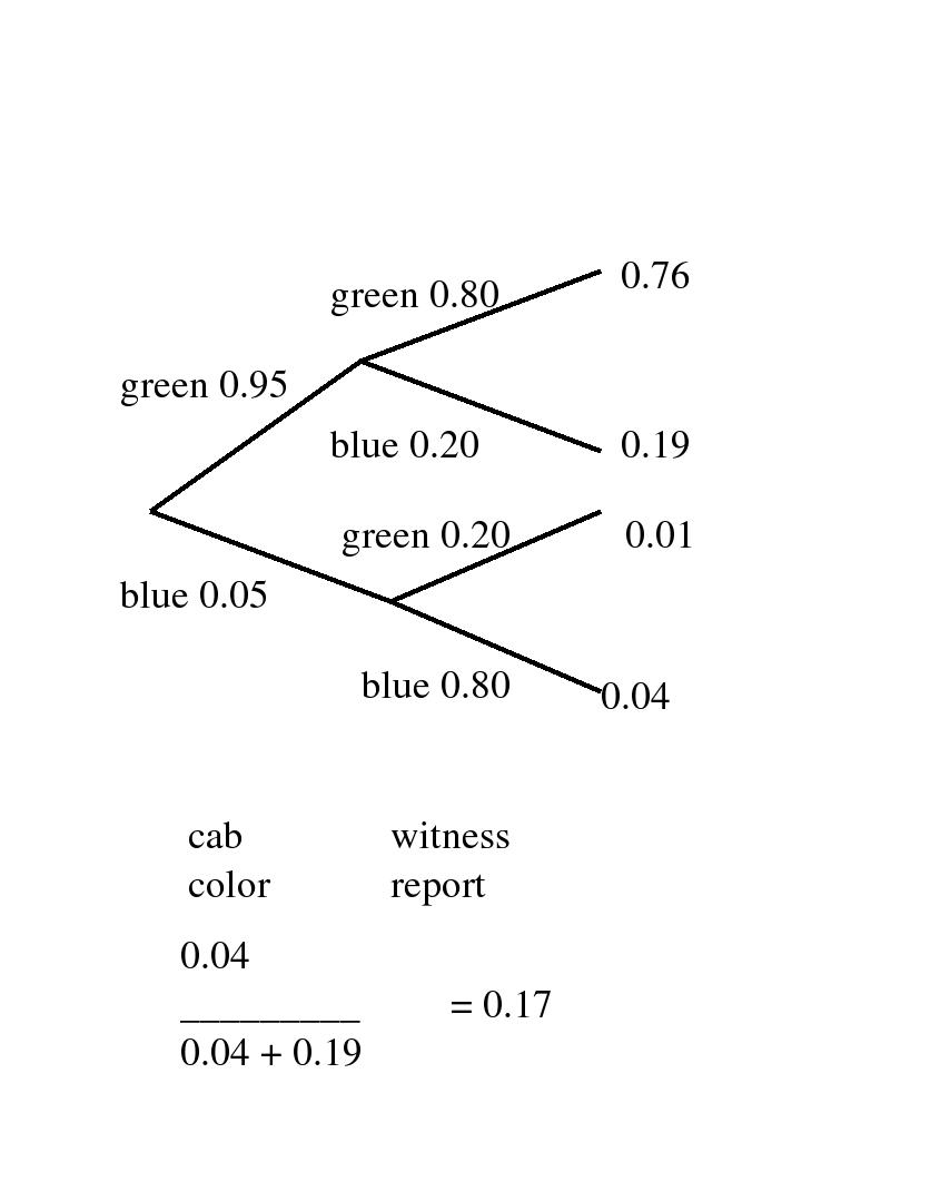
Another way to visually represent the calculations is with a box or Venn-like diagram.

Another Example of Reversing Probabilities

This example is adapted from: A First Course in Probability by Sheldon Ross, Macmillan, 1976, Chapter 3.3, Example 3c, page 52.

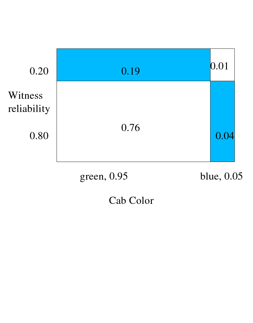
In answering a question on a multiple choice test, a student either knows the answer or the student just guesses. Suppose that the probability that the student knows the answer is 0.75, and the probability the student doesn’t know the answer and guesses is 0.25. Assuming that there are 5 choices for each multiple-choice question, then we take the probability that the student who guesses will be correct is 1/5 = 0.20. What is the conditional probability that the student knew the answer to a question given that the student answered it correctly?

Notice how the question asks the reverse of the simple conditional probability. Let C be the even that the student answers the question correctly. Let K be the probability the student knows the answer. Then the simple probability is . However, the problem posed here is , much different!

Here is a tree diagram of the same calculations:

A box diagram does not work well for this example, because the conditional probability of being correct given the prior information does not remain the same. That makes drawing the quartering box-line difficult.

Another Example of Reversing Probabilities with Three Events

This example is adapted from: A First Course in Probability by Sheldon Ross, Macmillan, 1976, Chapter 3, Problem 18, page 80.

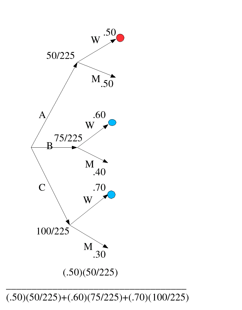
Stores A, B and C have 50, 75 and 100 employees respectively. and respectively, 50%, 60% and 70% of the employees are women. Resignations are equally likely among all employees, regardless of sex. One employee resigns and this is a woman. What is the probability that she works in store A?

Let W be the event that a woman employee resigns from anywhere, and let A, B and C denote the event that a randomly selected employee works at the respective store. Then Pr[A] = 50/225, Pr[B] = 75/225 and Pr[C] = 100/225. Likewise the probabilities of resignation of a woman from a store is given by the information to be Pr[W|A] = 0.50, Pr[W|B] = 0.60, and Pr[W|C] = 0.70 Then we can use Bayes Theorem (re-deriving it in the process of using it):

Here is a tree diagram of the same calculations:

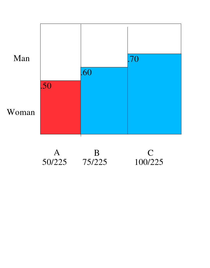
Another way to visually represent the calculations is with a box or Venn-like diagram.

Problems to Work for Understanding

[an error occurred while processing this directive] [an error occurred while processing this directive]

Last modified: [an error occurred while processing this directive]