Steven R. Dunbar
Department of Mathematics
203 Avery Hall
University of Nebraska-Lincoln
Lincoln, NE 68588-0130
http://www.math.unl.edu
Voice: 402-472-3731
Fax: 402-472-8466

Math 489/Math 889
Stochastic Processes and
Advanced Mathematical Finance
Dunbar, Fall 2009

__________________________________________________________________________

Solution of the Black-Scholes Equation

_______________________________________________________________________

Note: To read these pages properly, you will need the latest version of the Mozilla Firefox browser, with the STIX fonts installed. In a few sections, you will also need the latest Java plug-in, and JavaScript must be enabled. If you use a browser other than Firefox, you should be able to access the pages and run the applets. However, mathematical expressions will probably not display correctly. Firefox is currently the only browser that supports all of the open standards.

_______________________________________________________________________________________________

Rating

Mathematically Mature: may contain mathematics beyond calculus with proofs.

_______________________________________________________________________________________________

QuestionofDay

Question of the Day

What is the solution method for the Cauchy-Euler type of ordinary differential equation:

x^{2} \frac{d^{2} v}{d x^{2}} + a x \frac{d v}{d x} + b v = 0 ?

_______________________________________________________________________________________________

Key Concepts

We solve the Black-Scholes equation for the value of a European call option on a security by judicious changes of variables that reduce the equation to the heat equation. The heat equation has a solution formula. Using the solution formula with the changes of variables gives the solution to the Black-Scholes equation.
Solving the Black-Scholes equation is an example of how to choose and execute changes of variables to solve a partial differential equation.

__________________________________________________________________________

Vocabulary

A differential equation with auxiliary initial conditions and boundary conditions, that is an initial value problem, is said to be well-posed if the solution exists, is unique, and small changes in the equation parameters, the initial conditions or the boundary conditions produce only small changes in the solutions.

__________________________________________________________________________

Mathematical Ideas

Conditions for Solution of the Black-Scholes Equation

We have to start somewhere, and to avoid the problem of deriving everything back to calculus, we will assert that the initial value problem for the heat equation on the real line is well-posed. That is, consider the solution to the partial differential equation

\frac{\partial u}{\partial τ} = \frac{\partial^{2} u}{\partial x^{2}} - \infty < x < \infty, τ > 0 .

We will take the initial condition

u (x, 0) = u_{0} (x) .

We will assume the initial condition and the solution satisfy the following technical requirements:

$u_{0} (x)$ has no more than a finite number of discontinuities of the jump kind,
$lim_{| x | \to \infty} u_{0} (x) e^{- a x^{2}} = 0$ for any $a > 0$ ,
$lim_{| x | \to \infty} u (x, τ) e^{- a x^{2}} = 0$ for any $a > 0$ .

Under these mild assumptions, the solution exists for all time and is unique. Most importantly, the solution is represented as

u (x, τ) = \frac{1}{2 \sqrt{π τ}} \int_{- \infty}^{\infty} u_{0} (s) e^{- {(x - s)}^{2} ∕ 4 τ} d s

Remark. This solution can derived in several different ways, the easiest way is to use Fourier transforms. The derivation of this solution representation is standard in any course or book on partial differential equations.

Remark. Mathematically, the conditions above are unnecessarily restrictive, and can be considerably weakened. However, they will be more than sufficient for all practical situations we encounter in mathematical finance.

Remark. The use of $τ$ for the time variable (instead of the more natural $t$ ) is to avoid a conflict of notation in the several changes of variables we will soon have to make.

The Black-Scholes terminal value problem for the value $V (S, t)$ of a European call option on a security with price $S$ at time $t$ is

\frac{\partial V}{\partial t} + \frac{1}{2} σ^{2} S^{2} \frac{\partial^{2} V}{\partial S^{2}} + r S \frac{\partial V}{\partial S} - r V = 0

with $V (0, t) = 0$ , $V (S, t) ~ S$ as $S \to \infty$ and

V (S, T) = max (S - K, 0) .

Note that this looks a little like the heat equation on the infinite interval in that it has a first derivative of the unknown with respect to time and the second derivative of the unknown with respect to the other (space) variable. On the other hand, notice:

Each time the unknown is differentiated with respect to $S$ , it also multiplied by the independent variable $S$ , so the equation is not a constant coefficient equation.
There is a first derivative of $V$ with respect to $S$ in the equation.
There is a zero-th order term $V$ in the equation.
The sign on the second derivative is the opposite of the heat equation form, so the equation is of backward parabolic form.
The data of the problem is given at the final time $T$ instead of the initial time $0$ , consistent with the backward parabolic form of the equation.
There is a boundary condition $V (0, t) = 0$ specifying the value of the solution at one sensible boundary of the problem. The boundary is sensible since security values must only be zero or positive. This boundary condition says that any time the security value is 0, then the call value (with strike price $K$ ) is also worth 0.
There is another boundary condition $V (S, t) ~ S$ , as $S \to \infty$ , but although this is financially sensible, (it says that for very large security prices, the call value with strike price $K$ is approximately $S$ ) it is more in the nature of a technical condition, and we will ignore it without consequence.

We eliminate each objection with a suitable change of variables. The plan is to change variables to reduce the Black-Scholes terminal value problem to the heat equation, then to use the known solution of the heat equation to represent the solution, and finally change variables back. This is a standard solution technique in partial differential equations. All the transformations are standard, well-motivated, and well known.

Solution of the Black-Scholes Equation

First we take $t = T - \frac{τ}{(1 ∕ 2) σ^{2}}$ and $S = K e^{x}$ , and we set

V (S, t) = K v (x, τ) .

Remember, $σ$ is the volatility, $r$ is the interest rate on a risk-free bond, and $K$ is the strike price. In the changes of variables above, the choice for $t$ reverses the sense of time, changing the problem from backward parabolic to forward parabolic. The choice for $S$ is a well-known transformation based on experience with the Euler equidimensional equation in differential equations. In addition, the variables have been carefully scaled so as to make the transformed equation expressed in dimensionless quantities. All of these techniques are standard and are covered in most courses and books on partial differential equations and applied mathematics.

Some extremely wise advice adapted from Stochastic Calculus and Financial Applications by J. Michael Steele, [?, page 186], is appropriate here.

“There is nothing particularly difficult about changing variables and transforming one equation to another, but there is an element of tedium and complexity that slows us down. There is no universal remedy for this molasses effect, but the calculations do seem to go more quickly if one follows a well-defined plan. If we know that $V (S, t)$ satisfies an equation (like the Black-Scholes equation) we are guaranteed that we can make good use of the equation in the derivation of the equation for a new function $v (x, τ)$ defined in terms of the old if we write the old $V$ as a function of the new $v$ and write the new $τ$ and $x$ as functions of the old $t$ and $S$ . This order of things puts everything in the direct line of fire of the chain rule; the partial derivatives $V_{t}$ , $V_{S}$ and $V_{S S}$ are easy to compute and at the end, the original equation stands ready for immediate use.”

Following the advice, write

τ = (1 ∕ 2) σ^{2} (T - t)

and

x = log (\frac{S}{K}) .

The first derivatives are

\frac{\partial V}{\partial t} = K \frac{\partial v}{\partial τ} \cdot \frac{d τ}{d t} = K \frac{\partial v}{\partial τ} \cdot \frac{- σ^{2}}{2}

and

\frac{\partial V}{\partial S} = K \frac{\partial v}{\partial x} \cdot \frac{d x}{d S} = K \frac{\partial v}{\partial x} \cdot \frac{1}{S} .

The second derivative is

\begin{array}{l} \frac{\partial^{2} V}{\partial S^{2}} & = \frac{\partial}{\partial S} (\frac{\partial V}{\partial S}) \\ = \frac{\partial}{\partial S} (K \frac{\partial v}{\partial x} \frac{1}{S}) \\ = K \frac{\partial v}{\partial x} \cdot \frac{- 1}{S^{2}} + K \frac{\partial}{\partial S} (\frac{\partial v}{\partial x}) \cdot \frac{1}{S} \\ = K \frac{\partial v}{\partial x} \cdot \frac{- 1}{S^{2}} + K \frac{\partial}{\partial x} (\frac{\partial v}{\partial x}) \cdot \frac{d x}{d S} \cdot \frac{1}{S} \\ = K \frac{\partial v}{\partial x} \cdot \frac{- 1}{S^{2}} + K \frac{\partial^{2} v}{\partial x^{2}} \cdot \frac{1}{S^{2}} . \end{array}

The terminal condition is

V (S, T) = max (S - K, 0) = max (K e^{x} - K, 0)

but $V (S, T) = K v (x, 0)$ so $v (x, 0) = max (e^{x} - 1, 0)$ .

Now substitute all of the derivatives into the Black-Scholes equation to obtain:

K \frac{\partial v}{\partial τ} \cdot \frac{- σ^{2}}{2} + \frac{σ^{2}}{2} S^{2} (K \frac{\partial v}{\partial x} \cdot \frac{- 1}{S^{2}} + K \frac{\partial^{2} v}{\partial x^{2}} \cdot \frac{1}{S^{2}}) + r S (K \frac{\partial v}{\partial x} \cdot \frac{1}{S}) - r K v = 0 .

Now begin the simplification:

Isolate the common factor $K$ and cancel.
Transpose the $τ$ -derivative to the other side, and divide through by $σ^{2} ∕ 2$
Rename the remaining constant $r ∕ (σ^{2} ∕ 2)$ as $k$ . $k$ measures the ratio between the risk-free interest rate and the volatility.
Cancel the $S^{2}$ terms in the second derivative.
Cancel the $S$ terms in the first derivative.
Gather up like order terms.

What remains is the rescaled, constant coefficient equation:

\frac{\partial v}{\partial τ} = \frac{\partial^{2} v}{\partial x^{2}} + (k - 1) \frac{\partial v}{\partial x} - k v .

We have made considerable progress, because

Now there is only one dimensionless parameter $k$ measuring the risk-free interest rate as a multiple of the volatility and a rescaled time to expiry $(1 ∕ 2) σ^{2} T$ , not the original $4$ dimensioned quantities $K$ , $T$ , $σ^{2}$ and $r$ .
The equation is defined on the interval $- \infty < x < \infty$ , since this $x$ -interval defines $0 < S < \infty$ through the change of variables $S = K e^{x}$ .
The equation now has constant coefficients.

In principle, we could now solve the equation directly.

Instead, we will simplify further by changing the dependent variable scale yet again, by

v = e^{α x + β τ} u (x, τ)

where $α$ and $β$ are yet to be determined. Using the product rule:

v_{τ} = β e^{α x + β τ} u + e^{α x + β τ} u_{τ}

and

v_{x} = α e^{α x + β τ} u + e^{α x + β τ} u_{x}

and

v_{x x} = α^{2} e^{α x + β τ} u + 2 α e^{α x + β τ} u_{x} + e^{α x + β τ} u_{x x} .

Put these into our constant coefficient partial differential equation, cancel the common factor of $e^{α x + β τ}$ throughout and obtain:

β u + u_{τ} = α^{2} u + 2 α u_{x} + u_{x x} + (k - 1) (α u + u_{x}) - k u

Gather like terms:

u_{τ} = u_{x x} + [2 α + (k - 1)] u_{x} + [α^{2} + (k - 1) α - k - β] u .

Choose $α = - (k - 1) ∕ 2$ so that the $u_{x}$ coefficient is $0$ , and then choose $β = α^{2} + (k - 1) α - k = - {(k + 1)}^{2} ∕ 4$ so the $u$ coefficient is likewise $0$ . With this choice, the equation is reduced to

u_{τ} = u_{x x} .

We need to transform the initial condition too. This transformation is

\begin{array}{l} u (x, 0) & = e^{- (- (k - 1) ∕ 2) x - (- {(k + 1)}^{2} ∕ 4) \cdot 0} v (x, 0) \\ = e^{((k - 1) ∕ 2) x} max (e^{x} - 1, 0) \\ = max (e^{((k + 1) ∕ 2) x} - e^{((k - 1) ∕ 2) x}, 0) . \end{array}

For future reference, we notice that this function is strictly positive when the argument $x$ is strictly positive, that is $u_{0} (x) > 0$ when $x > 0$ , otherwise, $u_{0} (x) = 0$ for $x \leq 0$ .

We are in the final stage since we are ready to apply the heat-equation solution representation formula:

u (x, τ) = \frac{1}{2 \sqrt{π τ}} \int_{- \infty}^{\infty} u_{0} (s) e^{- {(x - s)}^{2} ∕ 4 τ} d s .

However, first we want to make a change of variable in the integration, by taking $z = (s - x) ∕ \sqrt{2 τ}$ , (and thereby $d z = (- 1 ∕ \sqrt{2 τ}) d x$ ) so that the integration becomes:

u (x, τ) = \frac{1}{\sqrt{2 π}} \int_{- \infty}^{\infty} u_{0} (z \sqrt{2 τ} + x) e^{- z^{2} ∕ 2} d z .

We may as well only integrate over the domain where $u_{0} > 0$ , that is for $z > - x ∕ \sqrt{2 τ}$ . On that domain, $u_{0} = e^{((k + 1) ∕ 2) \cdot (x + z \sqrt{2 τ})} - e^{((k - 1) ∕ 2) \cdot (x + z \sqrt{2 τ})}$ so we are down to:

\frac{1}{\sqrt{2 π}} \int_{- x ∕ \sqrt{2 τ}}^{\infty} e^{\frac{k + 1}{2} (x + z \sqrt{2 τ})} e^{- z^{2} ∕ 2} d z - \frac{1}{\sqrt{2 π}} \int_{- x ∕ \sqrt{2 τ}}^{\infty} e^{\frac{k - 1}{2} (x + z \sqrt{2 τ})} e^{- z^{2} ∕ 2} d z

Call the two integrals $I_{1}$ and $I_{2}$ respectively.

We will evaluate $I_{1}$ ( the one with the $k + 1$ term) first. This is easy, completing the square in the exponent yields a standard, tabulated integral. The exponent is

\begin{array}{l} ((k + 1) ∕ 2) (x + z \sqrt{2 τ}) - z^{2} ∕ 2 & = (- 1 ∕ 2) (z^{2} - \sqrt{2 τ} (k + 1) z) + ((k + 1) ∕ 2) x \\ = (- 1 ∕ 2) (z^{2} - \sqrt{2 τ} (k + 1) z + τ {(k + 1)}^{2} ∕ 2) + ((k + 1) ∕ 2) x + τ {(k + 1)}^{2} ∕ 4 \\ = (- 1 ∕ 2) {(z - \sqrt{τ ∕ 2} (k + 1))}^{2} + (k + 1) x ∕ 2 + τ {(k + 1)}^{2} ∕ 4 . \end{array}

Therefore

\frac{1}{\sqrt{2 π}} \int_{- x ∕ \sqrt{2 τ}}^{\infty} e^{\frac{k + 1}{2} (x + z \sqrt{2 τ})} e^{- z^{2} ∕ 2} d z = \frac{e^{(k + 1) x ∕ 2 + τ {(k + 1)}^{2} ∕ 4}}{\sqrt{2 π}} \int_{- x ∕ \sqrt{2 τ}}^{\infty} e^{\frac{- 1}{2} {(z - \sqrt{τ ∕ 2} (k + 1))}^{2}} d z .

Now, change variables again on the integral, choosing $y = z - \sqrt{τ ∕ 2} (k + 1)$ so $d y = d z$ , and all we need to change are the limits of integration:

\frac{e^{(k + 1) x ∕ 2 + τ {(k + 1)}^{2} ∕ 4}}{\sqrt{2 π}} \int_{- x ∕ \sqrt{2 τ} - \sqrt{τ ∕ 2} (k + 1)}^{\infty} e^{(- 1 ∕ 2) y^{2}} d z .

The integral can be represented in terms of the cumulative distribution function of a normal random variable, usually denoted $Φ$ . That is,

Φ (d) = (1 ∕ \sqrt{2 π}) \int_{- \infty}^{d} e^{- y^{2} ∕ 2} d y

I_{1} = e^{(k + 1) x ∕ 2 + τ {(k + 1)}^{2} ∕ 4} Φ (d_{1})

where $d_{1} = x ∕ \sqrt{2 τ} + \sqrt{τ ∕ 2} (k + 1)$ . Note the use of the symmetry of the integral! The calculation of $I_{2}$ is identical, except that $(k + 1)$ is replaced by $(k - 1)$ throughout.

The solution of the transformed heat equation initial value problem is

u (x, τ) = e^{(k + 1) x ∕ 2 + τ {(k + 1)}^{2} ∕ 4} Φ (d_{1}) - e^{(k - 1) x ∕ 2 + τ {(k - 1)}^{2} ∕ 4} Φ (d_{2})

where $d_{1} = x ∕ \sqrt{2 τ} + \sqrt{τ ∕ 2} (k + 1)$ and $d_{2} = x ∕ \sqrt{2 τ} + \sqrt{τ ∕ 2} (k - 1) .$

Now we must systematically unwind each of the changes of variables, from $u$ . First, $v (x, τ) = e^{(- 1 ∕ 2) (k - 1) x - (1 ∕ 4) {(k + 1)}^{2} τ} u (x, τ)$ . Notice how many of the exponentials neatly combine and cancel! Next put $x = log (S ∕ K)$ , $τ = (1 ∕ 2) σ^{2} (T - t)$ and $V (S, t) = K v (x, τ)$ .

The final solution is the Black-Scholes formula for the value of a European call option at time $T$ with strike price $K$ , if the current time is $t$ and the underlying security price is $S$ , the risk-free interest rate is $r$ and the volatility is $σ$ :

V (S, t) = S Φ (\frac{log (S ∕ K) + (r + σ^{2} ∕ 2) (T - t)}{σ \sqrt{T - t}}) - K e^{- r (T - t)} Φ (\frac{log (S ∕ K) + (r - σ^{2} ∕ 2) (T - t)}{σ \sqrt{T - t}}) .

Usually one doesn’t see the solution as this full closed form solution. Most versions of the solution write intermediate steps in small pieces, and then present the solution as an algorithm putting the pieces together to obtain the final answer. Specifically, let

\begin{array}{l} d_{1} & = \frac{log (S ∕ K) + (r + σ^{2} ∕ 2) (T - t)}{σ \sqrt{T - t}} \\ d_{2} & = \frac{log (S ∕ K) + (r - σ^{2} ∕ 2) (T - t)}{σ \sqrt{T - t}} \end{array}

so that

V_{C} (S, t) = S \cdot Φ (d_{1}) - K e^{- r (T - t)} \cdot Φ (d_{2}) .

Solution of the Black-Scholes Equation Graphically

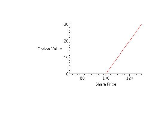
Consider for purposes of graphical illustration the value of a call option with strike price $K = 100$ . The risk-free interest rate per year, continuously compounded is 12%, so $r = 0.12$ , the time to expiration is $T = 1$ measured in years, and the standard deviation per year on the return of the stock, or the volatility is $σ = 0.10$ . The value of the call option at maturity plotted over a range of stock prices $70 \leq S \leq 130$ surrounding the strike price is illustrated in 1

Figure 1:

Value of the call option at maturity

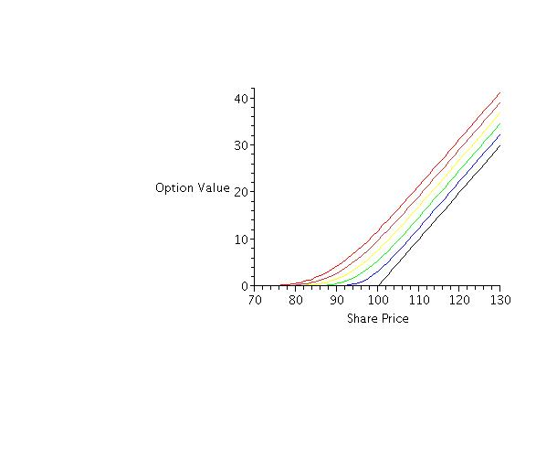
We use the Black-Scholes formula above to compute the value of the option prior to expiration. With the same parameters as above the value of the call option is plotted over a range of stock prices $70 \leq S \leq 130$ at time remaining to expiration $t = 1$ (red), $t = 0.8$ , (orange), $t = 0.6$ (yellow), $t = 0.4$ (green), $t = 0.2$ (blue) and at expiration $t = 0$ (black).

Figure 2:

Value of the call option at various times

Using this graph notice two trends in the option value:

For a fixed time, as the stock price increases the option value increases,
As the time to expiration decreases, for a fixed stock value price the value of the option decreases to the value at expiration.

We predicted both trends from our intuitive analysis of options. The Black-Scholes option pricing formula makes the intuition precise.

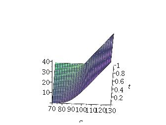
We can also plot the solution of the Black-Scholes equation as a function of security price and the time to expiration as value surface:

Figure 3:

Value surface from the Black-Scholes formula

This value surface shows both trends.

Sources

This discussion is drawn from Section 4.2, pages 59–63; Section 4.3, pages 66–69; Section 5.3, pages 75–76; and Section 5.4, pages 77–81 of The Mathematics of Financial Derivatives: A Student Introduction by P. Wilmott, S. Howison, J. Dewynne, Cambridge University Press, Cambridge, 1995. Some ideas are also taken from Chapter 11 of Stochastic Calculus and Financial Applications by J. Michael Steele, Springer, New York, 2001.

_______________________________________________________________________________________________

Problems to Work

Problems to Work for Understanding

Explicitly evaluate the integral $I_{2}$ in terms of the c.d.f. $Φ$ and other elementary functions as was done for the integral $I_{1}$ .
What is the price of a European call option on a non-dividend-paying stock when the stock price is $52, the strike price is $50, the risk-free interest rate is 12% per annum (compounded continuously), the volatility is 30% per annum, and the time to maturity is 3 months?
What is the price of a European call option on a non-dividend paying stock when the stock price is $30, the exercise price is $29, the risk-free interest rate is 5%, the volatility is 25% per annum, and the time to maturity is 4 months?
Show that the Black-Scholes formula for the price of a call option tends to $max (S - K, 0)$ as $t \to T$ .

__________________________________________________________________________

Books

Reading Suggestion:

__________________________________________________________________________

Links

Outside Readings and Links:

Cornell University, Department of Computer Science, Prof. T. Coleman Rhodes and Prof. R. Jarrow. Numerical Solution of Black-Scholes Equation, Submitted by Chun Fan, Nov. 12, 2002.
Monash University, Department of Mathematical Science, Eric. W. Chu. This link gives some examples and maple commands, Submitted by Chun Fan, Nov. 12, 2002.
An applet for calculating the option value. based on the Black-Scholes model. Also contains tips on options, business news and literature on options. Submitted by Yogesh Makkar, November 19, 2003.
ExcelEverywhere., a commercial application for spreadsheets on the Web. A sample spreadsheet based calculator for calculating the option values, based on Black-Scholes model. Submitted by Yogesh Makkar, November 19,2003

__________________________________________________________________________

I check all the information on each page for correctness and typographical errors. Nevertheless, some errors may occur and I would be grateful if you would alert me to such errors. I make every reasonable effort to present current and accurate information for public use, however I do not guarantee the accuracy or timeliness of information on this website. Your use of the information from this website is strictly voluntary and at your risk.

I have checked the links to external sites for usefulness. Links to external websites are provided as a convenience. I do not endorse, control, monitor, or guarantee the information contained in any external website. I don’t guarantee that the links are active at all times. Use the links here with the same caution as you would all information on the Internet. This website reflects the thoughts, interests and opinions of its author. They do not explicitly represent official positions or policies of my employer.

Information on this website is subject to change without notice.

Steve Dunbar’s Home Page, http://www.math.unl.edu/~sdunbar1

Email to Steve Dunbar, sdunbar1 at unl dot edu

Last modified: Processed from LATEX source on February 5, 2012